LCC Classifier Example

Preparing the data
Initializing and training the classifier
Plotting
Getting a response
Further information

Preparing the data

This example comes with the file 'circleHorseshoe1100.mat' which provides two variables, 'samples' and 'classified'.

load('cicleHorseshoe1100.mat');

While 'samples' is a 1100x2 matrix containing 1100 two-dimensional samples, 'classified' is a row-vector of length 1100 containing the individual class id (1, 2 or 3) of each sample.

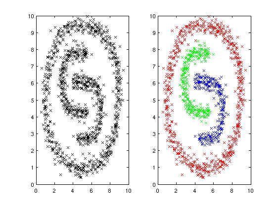
As you can see, the data forms a circle around two opposite horseshoes:

% Plain data
clf;
subplot(1, 2, 1);
plot(samples(1, :), samples(2, :), 'kx');

% Emphasize class ids
subplot(1, 2, 2);
plot(samples(1, classified == 1), samples(2, classified == 1), 'rx', ...
     samples(1, classified == 2), samples(2, classified == 2), 'gx', ...
     samples(1, classified == 3), samples(2, classified == 3), 'bx');

For further processing, the samples and class ids are permuted.

indices = randperm(size(samples, 2));

samples    = samples(:, indices);
classified = classified(:, indices);

Initializing and training the classifier

As a first step you are required to create a classifier configuration object. As no arguments are passed, all values will be set to their defaults.

config = createClassifierConfig();

To learn about the possible options look at the sourcecode of 'lcc/createClassifierConfig.m' and consult the literature given in the README document.

Using the configuration object a classifier can be constructed. Some of the samples and their respective class ids are used to setup the initial state.

classifier1 = newClassifier(samples(:, 1:50), classified(:, 1:50), [], config);

Since an incremental algorithm is used, the classifier can be updated by feeding even more samples and class ids.

classifier2 = updateClassifier(classifier1, samples(:, 51:1000), classified(:, 51:1000), []);

Plotting

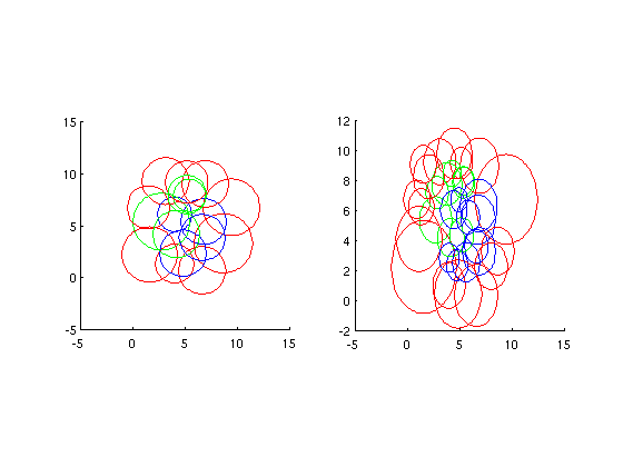
The function 'plotClassifier' displays the current state of the classifier by plotting all models using different colors to visualize their respective class id.

Note the apparent refinement after updating the classifier.

clf;
subplot(1, 2, 1);
plotClassifier(classifier1, 0, 'rgb');

subplot(1, 2, 2);
plotClassifier(classifier2, 0, 'rgb');

Getting a response

We use the 100 remaining samples that were not used during training to get a test response from the classifier. While there are different methods to get a response (just look at the getClassifierResponse* functions), this one is straightforward.

response = getClassifierResponse(classifier2, samples(:, 1001:1100));

The quality of the response can easily be evaluated. Note that the results are not strongly deterministic and thus may vary.

falseIndices = response ~= classified(1001:1100);
fprintf(1, 'False classifications: %d\n', sum(falseIndices));

False classifications: 0

Further information

All functions contain even more documentation. You can learn from the sourcecode or by using MATLAB's built-in help functionality by typing e.g. 'help newClassifier'.

You may also want to check out the literature given in the README document to learn about the methods behind the classifier and their various parameters.